Wow, now to make all the channels come out in surround sound…
Month: December 2013
Longer noise or sturdier mice?
Recordings with mics on the table:
- 105: 10s
- 106: 20s
- 107: 30s
- 108: 40s
- 109: 50s
Regular binaural recordings:
- 110: 50s front right
- 111: 40s front right
- 112: 30s front right
- 113: 30s back left
- 114: 40s back left
- 115: 50s back left
- 116: the actual moving target for 50s
And warning that came up when wavwrite was used to render the WAV files used for the recordings listed above…

Sound Card Problems?
Consumer products labelled 44.1 kHz MAY NOT BE SO! Its likely that our LMS filter was struggling to converge in on a moving target!
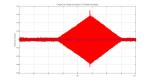
[ Insert: image of crosscorr beginning and end -> shift of about 80 samples ]
Working with RLS instead.
[ Read up on RLS ]
http://www.mathworks.com/matlabcentral/newsreader/view_thread/108767
Possible resolution:
dB: 10*log10(E^2)

8/90s recordings

Virtual surround sound, and some writing advise
Getting back to the commercialization post…
A lot of things have been going on! We even have a HowStuffWorks mentioning HRTFs, the Media Lab and some interesting sources.
And its not just the Media Lab, but CCRMA shows up too: [ Julius Smith ] -> a lot of resources!
So much to read – woo!
And a lecture on hash tables eventually led to:
Still no convergence…
So, I tried the 10 second noise sample
Good news: the cross-correlation was giving higher values.
-
- Source noise (w/ sines) & R1-0085 left ch.
-

- Source noise (no sines) & R1-0085 left ch. (actual)
-

- Removing R1-0085’s sines shifts the peak
And some zooming in fun (reverberation in the room?)

But I still didn’t have convergence. I thought about using Dr Anderson’s repeated filtration idea. First, I tried taking the last outputted weights and inputting them back into the algorithm for another run with the same data. The coefficients would bob up and down – start growing (giving the impression that we’ll have success) – and then soon after we entered the next run – the coefficients went back down to low values, and then repeat the process of eventually going back up again…
I think restarting the algorithm with a zero error might be causing this…
I also tried decreasing the step sizes with every run. But I don’t think that helped.
Then, I gave up and turned to the 20 second recording. First run, and the error started decreasing!!!!! But not much.
So, I decided the repeated filtration idea, however, this time, I just copied/concatenated the inputs with themselves to make them twice as big. Similar results as inputting initial weights for the case above.
(the animation below slows down right before the inputs get repeated, and we can see the coefficients becoming less exciting)
[click and refresh to re-run]

I changed the NLMS code to adjust the size of wAll (that collects the weights after every run) – I think we were just having a lot of zeros in wAll’s initial rows due to an indexing error I had made [not sure though]. I also added wAll as a function output. It made plotting/slowing down easier.
I think there’s something wrong with the code I added to the NLMS function. This is just weird…
Script used (along with the saved workspace with the source noise)
% Abhinav Uppal | ECE 3952 | Auditory Localization
%% Import WAV
fileNumStr = 'R1_0089'; % num2str(01)='1' and not '01'
file=sprintf('%s.wav',fileNumStr);

[yR01 fsR01 nBitsR01] = wavread(file);
yR01left  = yR01(:,1);
yR01right = yR01(:,2);

%% Sound Check | Imported File
recordedSignal = audioplayer(yR01, fsR01); % gets trunctated somehow. Use audioplayer.
play(recordedSignal);

%% Sound_check | noise source
srcSignal = audioplayer(noise10sined, fsNoise);
play(srcSignal)
clear srcSignal;

%% Did you see a sine?
figure(1);
window = 12;
spectrogram(yR01left, 2^12,[],2^12,fsR01,'yaxis')
title('Dec 5 | 44.1kHz | 84 big speaker (close) ','FontSize',16)

%% Remove most of the sine wave by looking at the spectrogram
noiseStart = 1.13;%1.5; % approx., using R1_0074
noiseEnd   = 21.35;%13; % approx., using R1_0074

figure(2);
yR01leftLessSine = yR01left(round(fsR01*noiseStart):round(fsR01*noiseEnd));
spectrogram(yR01leftLessSine,       2^12,[],2^12,fsR01,'yaxis')

%% Sound Check | Sine partially removed file
recordedSignal = audioplayer(yR01leftLessSine, fsR01);
play(recordedSignal);

%% Further refine the removal with cross corr
lol1 = noise20;

lol2StartFix = 0.07217;
lol2EndFix   = 0.14784;%trucate for same length

lol2Start   = lol2StartFix;
lol2End     = (noiseEnd -noiseStart) -lol2EndFix;
lol2        = yR01leftLessSine(round(fsR01*lol2Start):round(fsR01*lol2End));

figure(1)
crosscorr(lol1, lol2, 1e2)
% axis([3000,7000,-0.02,0.02])

%% Filtering
wZeros   = zeros(1,100);
w = wZeros;
mu = 0.5;
%%
% for i = 1:10
[~, ~, w, wAll4] = nlmsdva([lol2;lol2]', [lol1, lol1]', mu, wZeros); % actual weight unknown
% mu = mu/2;
% end

%% Manual checking wAll
clf;
axisYlow  = min(min(wAll4));
axisYhigh = max(max(wAll4));

%%
pause(3)
jumps = 5000;

for n=1:jumps:(1763902/2)
checker = stem(wAll4(n,:));
title(['Step # ' num2str(n) ' of 1763902'])
axis([1 100 axisYlow axisYhigh])
pause(.08)
delete(checker)
end

for joe=n:50:1763902/2 + 1000
checker = stem(wAll4(joe,:));
title(['Repeating Inputs & slow plotting -> Step # ' num2str(joe) ' of 1763902'])
axis([1 100 axisYlow axisYhigh])
pause(.08)
delete(checker)
end

for joe=1763902/2 + 1000:jumps:1763902
checker = stem(wAll4(joe,:));
title(['Fast forwarding, Step # ' num2str(joe) ' of 1763902'])
axis([1 100 axisYlow axisYhigh])
pause(.08)
delete(checker)
end
checker = stem(wAll4(end,:));
axis([1 100 axisYlow axisYhigh])
Shared sentiments
Its actually good to know that other people are in trouble too…

So if binaural is awesome…where are the commercial products?
Still having the convergence issue, I decided to look for an HRIR – to see what my expected filter would look like…
Hyperjumps:
[ Sony VPT ]
[ AuSIM ] [ skills ]
[ doi:10.1115/1.2203337 ] [ Martin, Gardner and KEMAR ]
The Sony’s page has some interesting things (data signal processing, gyroscopes in headphones…), but this takes us to the post title:
The benefits of this technology are, as stated before, the ability to achieve immersive life-like sound with directional quality through headphone reproduction.
The disadvantages are:

1) it is difficult to gain a clear sense of distance and directional positioning of the sound coming from the front.

2) The sound signals recorded using this method tend to sound high-pitched when reproduced through loudspeakers, thus,
   requiring two separate sources for headphone reproduction and loudspeaker reproduction. It is mainly for these
   weaknesses that this technology has failed to gain common acceptance despite of its excellent quality.
The front problem – I have had trouble with that. I have not really played back the sound on speakers – except by mistake – I don’t think that would produce any special effects unless we had the 3D3A stuff.
In fact, Choueiri told me that he can program in up to three ideal listening positions and cycle among them rapidly enough to produce all three at the same time.
And that is somewhat like my goal of quickly cycling between multiple HRIRs with a neural network…
And some more binaural fun…
Here’s something to consider for making music interesting:
- Lower frequencies stay in the middle
- Mid/higher frequencies go round and about
- It would be even better if we could have multiple instruments flying on their own!
First Successes with NLMS to-day/night!
Dr. Anderson suggested using his codes for NLMS so that the weights could be outputted with each step of the algorithm. (I don’t think there’s that option with MATLAB’s adaptfilt)
This post contains:
- The function for NLMS, with a helper animation function I added.
- A script that makes an input and filter at random, and then NLMS is used to arrive at this filter’s coefficients.
- Another script which takes this input – runs it first through a [1, -1] filter (not sure why there was a similar line in Dr Anderson’s code) – but net effect is that it takes longer for NLMS to converge.
I am including the function, both the scripts, and screen recordings (partial) of the results of running the code.
Its so cool to see the filter ACTUALLY adapt! Reminds me of Monte Carlo methods from BIOL 4105. So, lets start with the GIFs:
(click to view)
(Note: only some of the steps are actually shown)
-

- With the script’s orange line commented out.
-

- With the script’s orange line NOT commented out.
Here’s the function:
function [dhat,e,w] = nlmsdva(x,d,mu,w,varargin)
% x -> input vector, d -> desired output
% mu -> stepSize, w -> initial weights
% varargin for plotting
% {1}=actual wts, {2}=figID of the figure (default current+1)
% {3}=pause for animating wts. Avoid pause(0).
% {4}=perCent of steps to plot (default: plot 1% of the steps)

% NLMS implemented by:
% Dr David V Anderson
% School of Electrical and Computer Engineering
% Georgia Institute of Technology
%
% Helper function added by:
% Abhinav Uppal | ECE 3952

if (nargin < 4)
    % initial filter weight guess
    N = 10;
    w = zeros(1,N);
else
    N = length(w);
end

dhat = zeros(size(d));
e = zeros(size(d));
wAll = [w; zeros(length(x)-N+1,N)];

% now implement the adaptive filter
for n = N:length(x),
    xx = x(n:-1:n-(N-1));
    % produce filtered output sample
    dhat(n) = xx * w';
    % update the filter coefficients
    e(n) = d(n) - dhat(n);
    w = w+2*mu*xx*e(n)'/(xx*xx');
    wAll(n,:) = w;
end

if ~isempty(varargin)
    plotter(wAll,e,varargin)
end
end

function plotter(wAll,e,varargin)
plotMode = max(size([varargin{:}]));

wActual = varargin{1}{1};
[forLenX, N] = size(wAll);
lenX = forLenX +N -2; % -2 as wAll contains initial/input wts
wEnd = wAll(end,:);
if plotMode > 1
    figID = varargin{1}{2};
else
    figID = gcf + 1; % Hoping this would be free
end

figure(figID);
clf;

subplot(311)
stem(wActual,'r'); hold on;
predWts = stem(wEnd);
legend('actual wts', 'output wts')

subplot(312)
stem(wEnd(1:length(wActual))-wActual');
title('How good was it?')

subplot(313)
plot(10*log10(e.^2));
title('log10(error)')
axis([1,lenX,min(10*log10(e.^2)),max(10*log10(e.^2))])

if plotMode > 2
    pauseFor = varargin{1}{3};
    lowerBound = min(min(wAll));
    upperBound = max(max(wAll));

    subplot(311);
    delete(predWts);
    axis([1,N,lowerBound,upperBound])

    if plotMode > 3
        numSteps = round(forLenX*varargin{1}{4}/100);
    else
        numSteps = round(forLenX*1/100);
    end

    for i = round(linspace(1, forLenX, numSteps))
        child1 = stem(wAll(i,:));
        pause(pauseFor);
        title([num2str(i) ' of ' num2str(forLenX)])
        delete(child1);
    end
    stem(wEnd);
end
end
Script used – only one line differs for getting two different results (as highlighted in the code):
%% Screen Recording
clf([1,2]);
pause(10);
fprintf('Now!')
pause(2);

%% Seed
mySeed1 = rng(1,'v5uniform');
mySeed2 = rng(2,'v5uniform');

%% Dr Anderson's code (edited) for NLMS testing
sampLen = 10000;
rng(mySeed1);
x       = randn(sampLen,1);

beta    = 0.5;

% caps for vectors:
%                             X(n)
% W(n+1) = W(n) + beta.*e(n)--------
%                           ||X(n)||
%
% xe = sum(x.^2);% scaling factor?

figure(1);
plot(x);
title('input'); axis([0,1e4,-5,5]); pause(2);

x = filter(1,[1 -1],x); % imo FIR, no feedback -> high pass?
plot(x);
title('input: edited'); axis([0,1e4,-5,5]); pause(2);

% x = sqrt(xe)*x/sqrt(sum(x.^2)); % why so much work on input?
% figure(2);
% plot(x);
% title('input: scaled & normalized')
% axis([0,1e4,-5,5])
% pause(1);

rng(mySeed2);
h = rand(10,1);
d = filter(h,1,x);
figure(1);
plot(d);
title('output'); axis([0,1e4,-5,5])
%x = x+0.001*randn(size(x));

[dhatn,en,wn] = nlmsdva(x',d,beta,zeros(1,20),h,2,0.01,10);
